2.1     Decibel Matching and Pink Noise

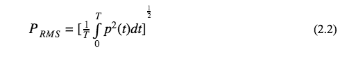
Whether a signal is digital or analog, there is decibel level associated with the signal. A decibel is a logarithmic ratio comparing the voltage to a reference voltage. The threshold for human hearing is considered 0dB which is known as the acoustic sound pressure reference (Wolfe, Joe). Sound pressure, p, is the sound field quantity measured in decibels (or dB-SPL). This can be measured through the formula below.

The preference is equal to 20 micropascal and pRMS is the RMS value of the acoustic sound pressure.

Decibel meters are tools that measure sound pressure levels in dB SPL. They typically are assignable with weighting A or C that apply filters. These weighting filters will help compensate for what a human ear hears. These weighting charts can be seen in the figure below. For our data to remain constant with what is happening in reality, the digital intensity of the sound has to match the acoustic sound intensity measured at the microphone position.

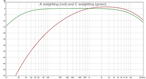
Figure 2.1: Decibel Meter A Weighting VS. C Weighting

To match the decibel levels a test tone of pink noise will be played through the speakers. Pink noise is a random noise that has equal energy per octave and is used to compensate for the human inability to hear lower frequencies in comparison to higher frequencies. It is similar to applying a long exaggerated low pass filter on white noise. White noise is equal energy per frequency. This long exaggerated low pass filter of the pink noise signal creates a random signal passing only the audible range of frequencies 20Hz-20kHz. The algorithm to generate pink noise was first demonstrated in matlab and then converted to C++ coding. The pink noise algorithm written in 2 matlab codes can be found in appendix A.

2.2 Frequency Sweep Generation

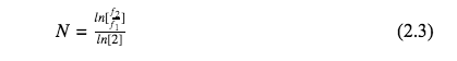
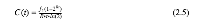
The frequency sweep, just like the pink noise file, was a code written in C++ that was then implemented into our loop function of our code. The frequency sweep depends on many factors. First and foremost the starting and ending frequency of the sweep along with the starting and ending time. In the equations below C is the accumulated cycles and R is the rate at which the frequency sweeps fromf1 to f2. The number of octaves in the sweep is represented with N. The final equation represents the amplitude of the sine sweep signal.

The logarithmic sweep can now be set up by defining the number of octaves N to then solve for the sweep rate R. The sweep rate, to be more specific, refers to the number of octaves per second.

The accumulated cycles are the progression of the frequencies comprised in the sweep. This function is dependent on the sweep rate and is a function of time.

The accumulated cycles will be the frequency of the final sine wave equation. The amplitude response will a sine function with the accumulated cycles in place of the frequency of the sine function.

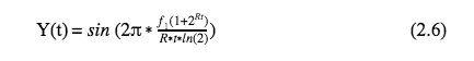
This will create a signal where the frequency builds to oscillate faster and faster. The time domain signal can be seen in figure 2.2 below for a 5 second analysis. Our tonesweeps are all 30 seconds which allows for an abundant amount of samples for the more accuracy.

Figure 2.2: Tonesweep Time-Domain Plot

2.3 Filter Design

In order to design a correction filter a series of bandpass and band-stop filters have to be generated. Equalization (EQ) is pretty typical in the audio industry but even the most sophisticated equalizer is limited to 8 or 9 bands of parametric EQ. The resulting curves can be seen below in figure (2.3). In blue is the original response, in yellow is the equalization curve, and in green the resulting curve when the original and EQ curve are summed together.

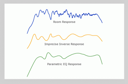
Figure 2.3: Resulting Signals for Applying Multi-band Parametric EQ

Our sophisticated room correction software has almost an unlimited amount of parametric equalizers. These filters are then summed together in parallel which means they are summed together at once. A demonstration of this can be seen below in figures (2.4) and (2.5). For figure (2.5), in blue is the original response, in yellow is the equalization curve, and in red the resulting curve when the original and EQ curve are summed together.

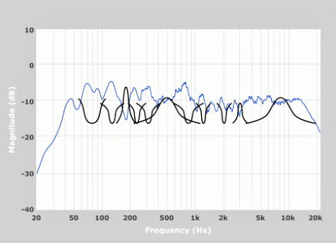
Figure 2.4: Multi-band Parametric EQ

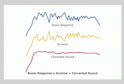
Figure 2.5: Individual Signals for Applying Precise Inverse Correction Filter

In figure (2.5) below the original signal can be compared to the resulting correction filter. The correction filter is formed from all of the filters generated, which are almost an exact inverse curve from the original frequency response. The point in which original signal peaks the filter has a valley and vice versa all throughout the spectrum.

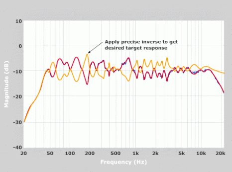
 Figure 2.6: Original Signal VS Precise Inverse Correction Filter

    To create these parallel IIR filters that make up the final room correction filter, several parameters must be obtained. First, identify if it a band pass or stop-band filter with either a positive or negative gain applied to the signal. If a positive gain is needed, we apply a pass band filter with the gain needed. If it is a negative gain we will apply a band stop filter with the appropriate gains needed, which is explained in detail in chapter 3.3.

The center frequency of the filter and the bandwidth are also very important factors to take into consideration. The typical radian frequency formula for the center frequency:

then becomes,

and the center frequency is divided by the sampling frequency. The bandwidth in radians is also to be inversely proportional to the sampling frequency.

Sometimes, like in audio applications, the bandwidth is referred to as “Q” which is short for quiescent point. These are the points in the signal that reach 0.707 of the signal peak and represent the cutoff frequencies of a filter. Both band pass and stop-band filters have two of these points on either side of the center frequency.

After determining these parameters through our algorithm that detects the amplitude peaks and valleys of the frequency spectrum, the IIR filters will be generated. IIR filters are infinite impulse response filters that can be applied in many applications, however, filtering audio is the most common.

Continuing the design of the IIR filter, we establish that our filter will be designed around the center frequency which will be identified as c=0 for digital language. The surrounding filter samples are shifted to left or right of 0. This can be seen in the difference equation 2.14.

The basic transfer function for all of the filter were derived from analog prototypes using the Bilinear Transformation (BLT).

There are 6 coefficients in this transfer function so we will normalize it by equating

to equal

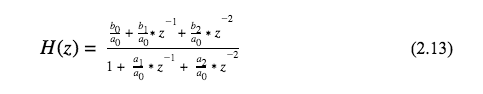
after the normalization of a0.

The most straightforward approach would be “Direct Form 1”

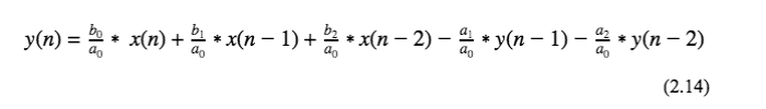
But before substituting the particular filter coefficients into the equation (2.10), we need to calculate the auxiliary variable .

                            

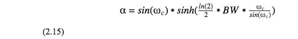
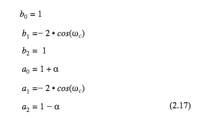
The coefficients for the bandpass filter are as follows.

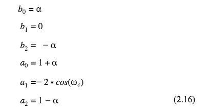
The coefficients for the stop-band filter are similar to the bandpass coefficients but create an upside down bell curve.

The s-domain of the transfer function, after simplification, becomes

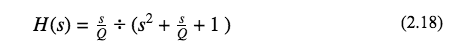
and

for the stop-band filter. The bilinear transformation substitutes

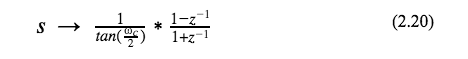
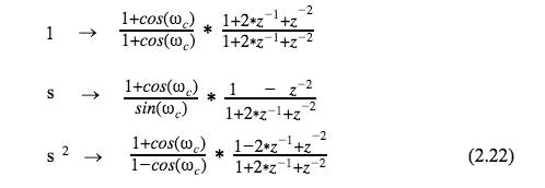
which will use the trig identities

in the resulting z-transformations for the filters transfer functions

3.1

The Fast Fourier Transform (or FFT) that is used is referenced as an FFT1024 object for several reasons. First being that it samples the audio 1024 times and then displays a line of data, this causes the serial monitor to update with new FFT values 86 times per second. It is also reads 1024 samples of the frequency spectrum. So during the time it takes to sample the time domain signal 1024 times it will read 512 bins of frequencies 43Hz apart, and it will do this twice equaling 1024 frequency bins of data.

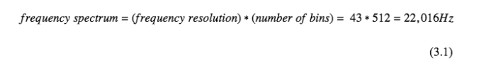
The frequency resolution is restricted due to processing memory available on the microcontroller. With an upgraded processor and RAM the FFT algorithm could handle more values which could significantly reduce the frequency resolution. The FFT is applied twice per 1024 samples to avoid any error. The first FFT will sample the frequencies 1024 times beginning at time 0. The second FFT, also 1024 samples, will have a delay of 512 samples and therefore creating a 50% overlap in the FFT sampling. This can be seen in figure 3.1 below.

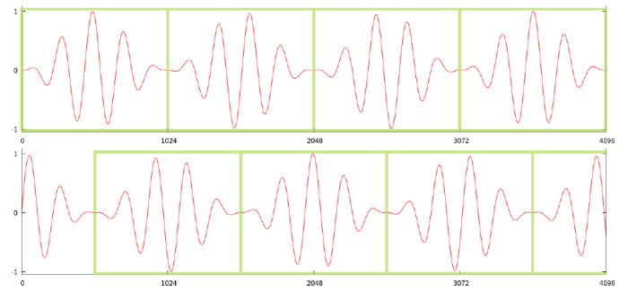Figure 3.1: Digital Sampling Example

Our microcontroller will display 16 values that correspond to 16 individual frequency bins. Most all of them are grouped together because of the logarithmic pattern of the frequency axis. After the third frequency bin the frequencies begin to group together in order to follow the logarithmic pattern of the frequencies. Next to the frequency axis it will display the time domain signal in a graphical display and then print the associated volume number values along the far right side of the display of Arduino’s Serial Monitor.

Figure 3.2: Serial Monitor Displaying Data

All of the values are normalized and displayed in dBFS, from 0 to 1.

3.2 Collecting Data

As mentioned before, the controller will first play some pink noise for 15 seconds and record the average amplitude of the time domain signal. The average amplitude will be our unity gain target line for our filters. In figure 3.3 below the characters on the left are a graphical representation of the time domain signal printing vertically. Just to the right of the graphical representation of the time domain is the amplitude of the signal in dBFS and then to the far right it is keeping track of the CPU usage since we were having issues with overloading it with data. After the pink noise is done and the average amplitude has been calculated the controller will send a tonesweep signal directly to the FFT to simulate a perfect world scenario for the tonesweep to be compared to after the filters have been applied.

Figure 3.3: Pink Noise While Analyzing the Time Domain Signal

In figure 3.4 below it can be seen that there are 16 bins of changing numbers that represent the frequency spectrum from 0Hz-18kHz. The first bin represents 0Hz and can always be ignored. To the right of the frequency spectrum is the same time domain analysis as before with the graphical representation next to the decibels associated. In this perfect signal there is a constant tone coming into the left channel of the peak analysis. Next we will play the tonesweep through the speakers without any filters to analyze the distorted signal caused by the frequency responses of the speakers, room, and microphone.

Figure 3.4: Perfect Tonesweep

The data in figure 3.5 is displaying the data of the tonesweep through the speakers and captured through the microphone. The data from this part of the analysis will have a similar layout as figure 3.4. First is the 16 bin FFT analysis followed by the time domain analysis. At the end of all the tonesweeps it will print the max value received in each frequency bin. This line of data that will used as the frequency response for all 3 tonesweeps.

Figure 3.5: Frequency Analysis Before Filtering

Figure 3.6 is the final tonesweep analysis where the tonesweep signal is passed through the generated filters and gains, then played through the speaker and captured through the microphone to display the frequency domain. The filters use a lot of processing power and therefore the time domain was not analyzed. Figure 3.7 shows a plot of the frequency spectrum of the analysis conducted.

Figure 3.6: Frequency Analysis After Filtering

3.3 How the Filters are Generated and Used

Due to limitations of the microcontroller, we were only able to use a limited amount of filters. Originally there were a total of 40 parallel filters per output channel, 80 filters total. For each output channel there were 20 bandpass filters and 20 stop-band filters. Since the frequency response is displayed in 16 bins and we know the bandwidth of the displayed values, the filters used are set up with a fixed center frequency and bandwidth. We chose to filter the signal according to what is being analyzed. The microcontroller will look at whether the analyzed data is above or below the threshold set up by the pink noise and will decide to use a bandpass filter or a band-stop filter. Then it will determine how much gain needs to be added in order to adjust the frequency response.

Keeping in mind that the filters are set to unity gain the filters will have gain adjustments through the Teensy digital mixer object. However the stop-band filter naturally is 0 at the center frequency and a 1 everywhere outside of the bandwidth and therefore positive gain must be added. For instance, the data is normalized with values from 0 to 1 (floating point). If our unity gain line was 0.70 and we read a 0.81 during the second tonesweep analysis that plays through the speakers without filters, we would know that we would need a cut of 0.11. However, since the stop-band filter would completely eliminate that frequency, we would apply a positive gain of 0.89.

This will compensate for the effects of the stop-band filter completely eliminating that frequency.

The filters were tested in Matlab using the transfer function seen in equation 2.13 in chapter 2. They were tested by running a low resolution audio test signal through the filter and a plotted the frequency response of the filter with the phase response of the filter found in figure 3.7 below. The bandpass filter has a bell curve with a center frequency of 1200 Hz.

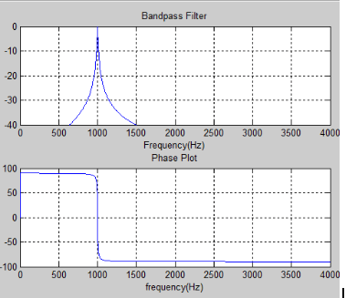
Figure 3.7: Bandpass Filter in Matlab

The time domain of the test signal is then plotted before and after the filter is applied in figure 3.8. It can be seen that after the filter is applied that the noise is reduced and the difference is certainly audible. It can be seen in figure 3.9 below that the frequency response of the filtered signal only reflects the frequencies passed by the filter in comparison to the original frequency response.  The Matlab code for both the bandpass filter can be seen in Appendix B.

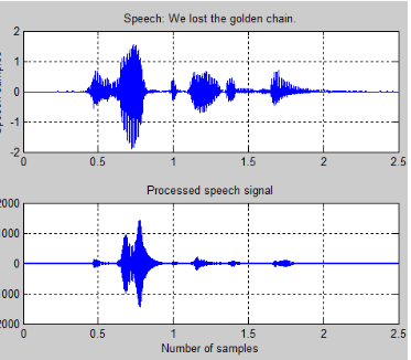
Figure 3.8: Matlab Audio Signal Before and After Filtering

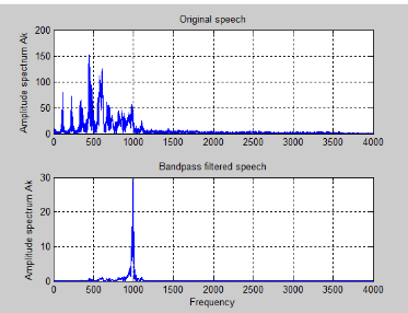
Figure 3.9: Bandpass Frequency Response

A separate code was created for Matlab to simulate the results of the band- stop filter used in this project. The band-stop filter will reject the frequencies at the center frequency and pass all other frequencies. The bode plot of the band-stop filter centered around 600Hz with a bandwidth of 200Hz can be seen below in figure 3.10. The Matlab code for both the band-stop filter can be seen in Appendix C.

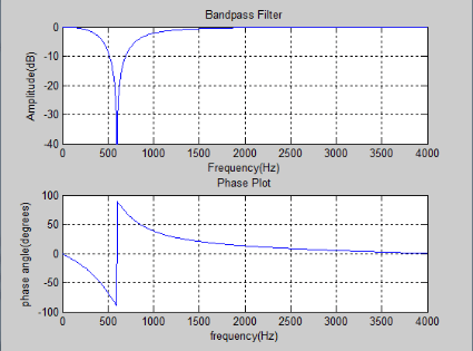
Figure 3.10: Band-stop Filter in Matlab

3.4 System Overview

The RTRC was designed with the intention of not being connected to a computer and therefore we made a regulated power supply that will take the standard 120V AC signal from the typical power outlet and provide safe regulated power for the entire device. It was simulated in Multisim software to ensure the correct voltage is provided. The -15V was originally generated for an op-amps for the passing of the audio signal in and out of the microcontroller. After switching to Teensy with the audio shield the same op-amp was already provided. The power regulating circuit can be seen below in figure 3.11 with the simulation results of the output.

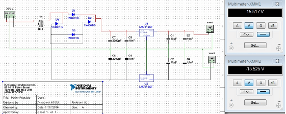
Figure 3.11: Power Regulating Circuit

This circuit then has a power regulator for the Teensy’s 5V input source. This is to power the Teensy without a computer, which would normally display the data. The device will work do it’s job with our without a computer. Also an LED is connected to this voltage regulator for the indication that the device is ON or OFF.

The Teensy audio shield sits right on top of the Teensy microcontroller, pin for pin. From this audio shield we transmit and receive the audio signals. This shield is fantastic for audio applications. It has on-board ADC’s and DAC’s to convert the signals to and from the digital domain. The circuit doesn’t end with only the analog parts.

We also created a digital circuit using Teensy’s audio GUI tool. This helped us create a digital circuit to control signal flow for the digital signal. The digital circuit that can be seen below in figure 3.12 is the original circuit created. But of course Teensy 3.2 couldn’t handle that many filters so we shortened the circuit in order to for the Teensy to process the large amount of data. So we just “commented out” a good majority of the filters from this digital circuit, that way we can easily expand when the time is right. Figure 3.13 contains the circuit surrounding the microcontroller and figure 3.14 shows the block diagram of the entire circuit.

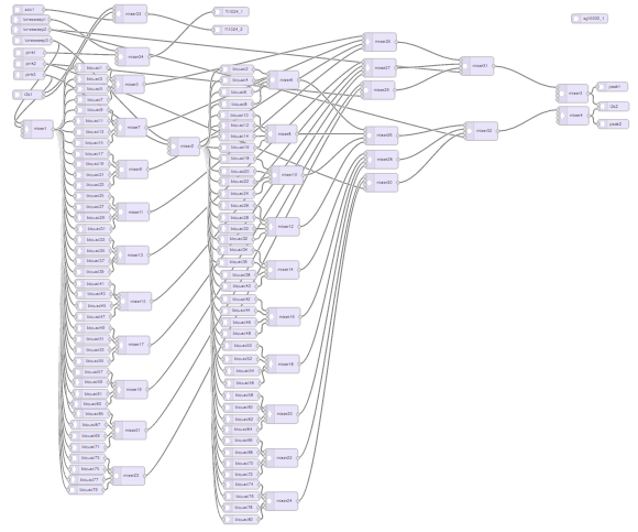
Figure 3.12: Digital Circuit for Teensy

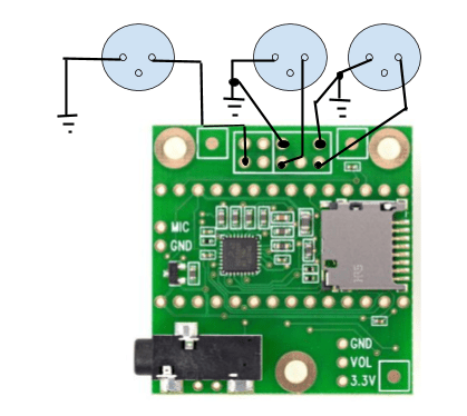
Figure 3.13: Microcontroller Circuit

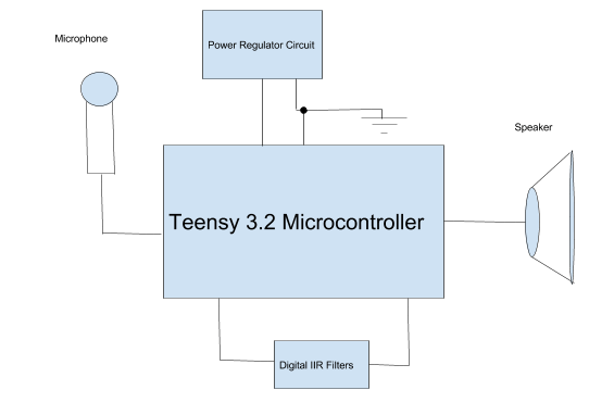
Figure 3.14: Block Diagram

3.5 Results and Discussion

The RTRC design was a success. The limitations of the Teensy only allowed for a couple of filters and therefore we could only filter a portion of the audio spectrum, 300Hz to 3kHz. In this frequency range the RTRC was able to filter the audio signal to allow for an audio signal to pass with a smoother response. This idea can be expanded upon for future use as explained later in chapter 5.

We ran the total analysis 10 times while moving the microphone around and plotted the frequency analysis. Each time the microphone was moved to a different location within the room the frequency response will change. Each time the signal changed the RTRC compensated and smoothed the signal according to the pink noise level measured. The smoothed signal becomes a closer example to the “perfect tonesweep” we analyze shortly after playing the pink noise signal. As seen in figure 2.2 above, the amplitude of the frequency sweep remains constant throughout the spectrum. Figures 3.15 through figure 3.24 are a series of 10 sweeps that reflect the different microphone position within the room. Each plot shows the corrected signal is a smoother response.

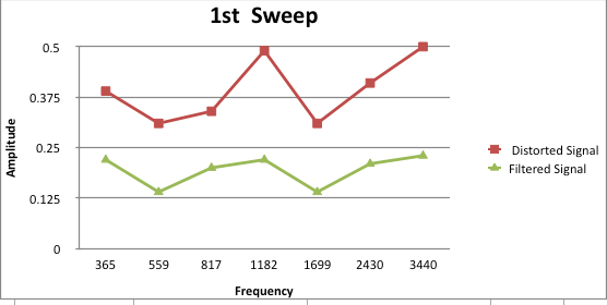
Figure 3.15: Analysis 1

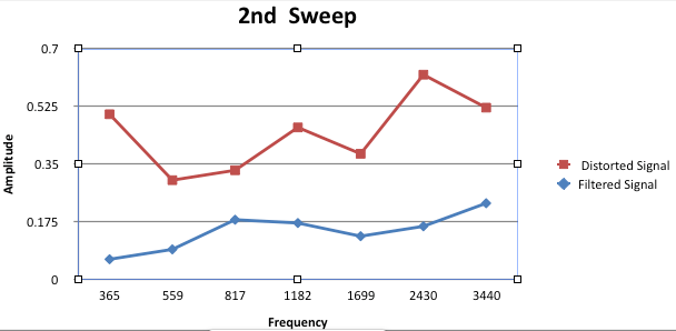
Figure 3.16: Analysis 2

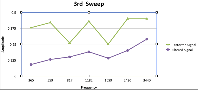
Figure 3.17: Analysis 3

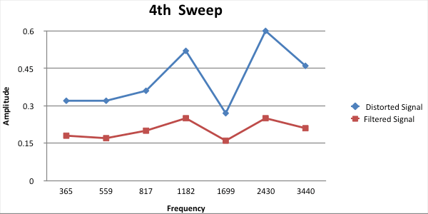
Figure 3.18: Analysis 4

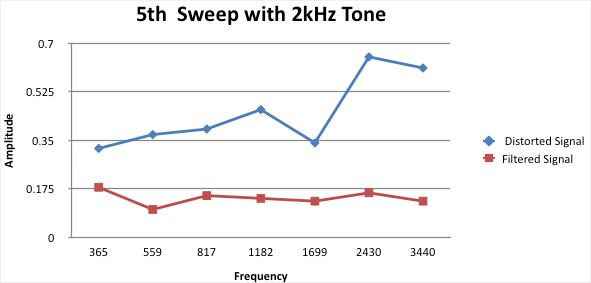
Figure 3.19: Analysis 5

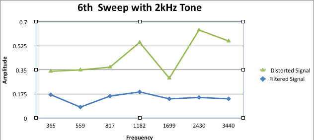
Figure 3.20: Analysis 6

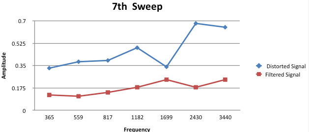
Figure 3.21: Analysis 7

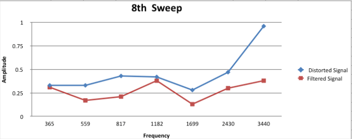
Figure 3.22: Analysis 8

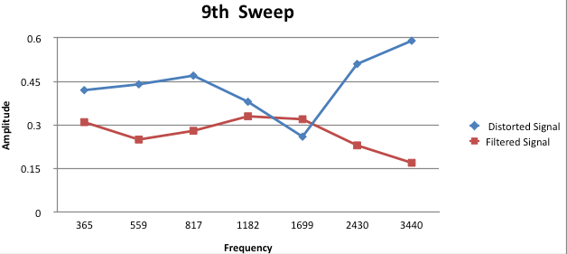
Figure 3.23: Analysis 9

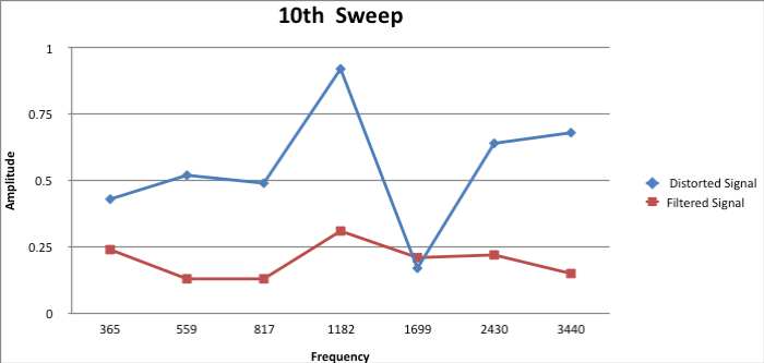
Figure 3.24: Analysis 10

As it can be seen in these 10 graphs, the RTRC is doing its job. It is tastefully applying digital filters to smooth the frequency response at the listening position. The circuit design and coding all came together for some immaculate results. I would use this system on my own home theater system to obtain these type of results! The potential for this design is endless since everyone loves clean and smooth audio whether they know it or not.

Summary and Conclusions

The RTRC is a standalone device that analyzes an audio system and provide a correction filter to send to any amplifier for a set of speakers chosen by the user. The theory seemed to match up with real world application with each portion of our project. Due to limitations of the chosen microcontroller it is far from being the ideal room analyzer. However this project was challenging and has taught us a great deal about digital signal processing and how send an analog signal through a microcontroller in the digital domain and back into an analog and acoustical signal.

We did encounter many problems along the way. One of the biggest mistakes we made was choosing the wrong microcontroller to begin with. The Teensy 3.2 was not our first choice but it did turn out to be the better choice for this device. Our first choice was an arm embedded FRDM-k22f. We originally thought it would handle our project with ease since it had the capability of high sample rates with a 16 bit depth and had a lot of on-board memory. We quickly found out that it was a really bad choice when we couldn’t upload a simple test code. It turns out that it was due to static electricity making contact with the controller, creating a short circuit. We went through 2 of them before finding out that static electricity could even be an issue. It was an easy decision at that point to use a different microcontroller for the project. The Teensy is a very powerful microcontroller in such a small package.

The challenging nature of this complex DSP unit was most rewarding when we were able to get it to work. We both learned a great deal throughout all of our studies and countless hours of research to get the project to where it currently is. The Teensy 3.2 still isn’t powerful enough to handle the complex operations we are demanding of it. Fortunately there is a solution, Teensy has just released a new and even more powerful microcontroller, the Teensy 3.6 microcontroller. It has only been on the market since September 2016 and therefore has bugs to work out. After the bugs have been addressed, it should resolve a number of issues for us since the RAM is quadrupled as well as the on-board memory.

There are certainly real time analyzer (RTA) instruments and softwares out on the market and there are even sophisticated digital audio workstations (DAW’s)  that you can save correction filters for the system to send an audio signal through. However, these systems are very expensive and dependent on a computer with sophisticated software to communicate with the speakers. Most home theatre systems do not even have the ability to connect to a computer. This stand-alone device will eliminate the need to connect to a computer and could be manufactured at a low enough cost to make it affordable for the average consumer.

We stepped out of our comfort zone in taking on this project for senior design class, but managed to make something of it. It was very rewarding to have accomplished our goals in designing an automatic equalizer for audio signals. The reward will only be that much sweeter when we can launch it as a product on the audio electronics market.

5.2     Suggestions for Future Work

Although we were successful in filtering the audio signal, here are certainly many things that can be done to improve the RTRC. First and foremost, by extending the limitations of the RAM and onboard memory of our Teensy 3.2 microcontroller, we could expand the number of filters. Potentially the number of filters could be upwards of 80 filters. Also the frequency resolution of our FFT could be dramatically decreased therefore improving the accuracy of our analysis. This in turn would also give us the ability to look at more frequency bins.

The other modification that can be done is something we planned to accomplish but ran out of time to add. The addition of the second audio shield to pass audio through the filters. The second audio shield will only add double the I/O. All in all, we could replace the microcontroller with the Teensy 3.6 with two audio shields and it should fix everything. After those few modifications, I believe the RTRC could become a sellable item.